Subex Blog

Introduction : Hyperparameter optimization is the science of tuning or choosing the best set of hyperparameters for a learning algorithm. A set of optimal hyperparameter has a big impact on the performance of any machine learning algorithm. It is one of the most time-consuming yet a crucial step in machine learning training pipeline. A Machine learning model has two types of tunable parameter :

• Model parameters
• Model hyperparameters

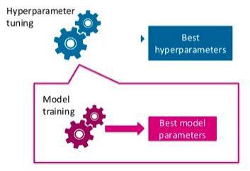
Model parameters vs Model hyperparameters (source) Model parameters are learned during the training phase of a model or classifier. For example :

• coefficients in logistic regression or liner regression
• weights in an artificial neural network

Model Hyperparameters are set by user before the model training phase. For example :

• ‘c’ (regularization strength), ‘penalty’ and ‘solver’ in logistic regression
• ‘learning rate’, ‘batch size’, ‘number of hidden layers’ etc. in an artificial neural network

The choice of Machine learning model depends on the dataset, the task in hand i.e. prediction or classification. Each model has its own unique set of hyperparameter and the task of finding the best combination of these parameter is known as hyperparameter optimization. For solving hyperparameter optimization problem there are various methods are available. For example :

• Grid Search
• Random Search
• Optuna
• HyperOpt

In this post, we will focus on Optuna library which has one of the most accurate and successful hyperparameter optimization strategy. Optuna : Optuna is an open source hyperparameter optimization (HPO) framework to automate search space of hyperparameter. For finding an optimal set of hyperparameters, Optuna uses Bayesian method. It supports various types of samplers listed below :

• GridSampler(using grid search)
• RandomSampler(using random sampling)
• TPESampler (using Tree-structured Parzen Estimator algorithm)
• CmaEsSampler ( using CMA-ES algorithm)

Use of Optuna for hyperparameter optimization is explained using Credit Card Fraud Detection dataset on Kaggle. The problem statement is to classify a credit card transaction fraudulent or genuine(binary classification). This data contains only numerical input variables which are PCA transformation of original features. Due to confidentially issues, the original features and more background information about the data are not available. In this case, we have used only a subset of the dataset to speed up the training time and to ensure the two different classes reach a perfectly balance. Here, the sampling method used is TPESampler . 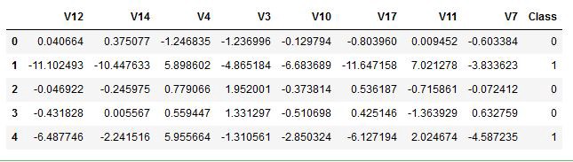A subset of a dataset is shown in the figure below : A subset of Credit Card Fraud Detection dataset Importing required packages : import optuna from optuna import Trial, visualization from optuna.samplers import TPESampler from xgboost import XGBClassifier Following are the main steps involved in HPO using Optuna for XGBoost model:

1. Define Objective Function : The first important step is to define an objective function. The objective should be to return a real value which has to minimize or maximize. In our case, we will be training XGBoost model and using the cross-validation score for evaluation. We will be returning this cross-validation score from an objective function which has to be maximized.
2. Define Hyperparameter Search Space : Optuna supports five kind of hyperparameters distribution, which are given as follows :

• Integer parameter: A uniform distribution on integers. n_estimators = trial.suggest_int(‘n_estimators’,100,500)
• Categorical parameter: A categorical distribution. criterion = trial.suggest_categorical(‘criterion’ ,[‘gini’, ‘entropy’])
• Uniform parameter: A uniform distribution in linear domain. subsample = trial.suggest_uniform(‘subsample’ ,0.2,0.8)
• Discrete-uniform parameter: A discretized uniform distribution in linear domain. max_features = trial.suggest_discrete_uniform(‘max_features’, 0.05,1,0.05)
• Loguniform parameter: A uniform distribution in log domain. learning_rate = trial.sugget_loguniform(‘learning_rate’ : 1e-6, 1e-3)

The below figure shows the objective function and hyperparameter for our example. Objective Function

3. Study Objective : We have to understand some important terminologies mentioned in their docs, which will make our work easier. These are given as follows :

• Trial : A single call of the objective function
• Study : An optimization session, which is a set of trails
• Parameter : A variable whose value is to be optimized such as value of “n_estimators”

The Study object is used to manage optimization process. Method create_study() returns a study object. A study object has useful properties for analyzing the optimization outcome. In method of create_study(), we have to define the direction of objective function i.e. “maximize” or “minimize” and sampler for example TPESampler(). After creating study, we can call Optimize().

4. Best Trial and Result : Once the optimization process completed then we can obtain the best parameters value and the optimal value of the objective function.

Best trial: score 0.9427118644067797, params {‘n_estimators’: 396, ‘max_depth’: 6, ‘reg_alpha’: 3, ‘reg_lambda’: 3, ‘min_child_weight’: 2, ‘gamma’: 0, ‘learning_rate’: 0.09041583301198859, ‘colsample_bytree’: 0.45999999999999996}

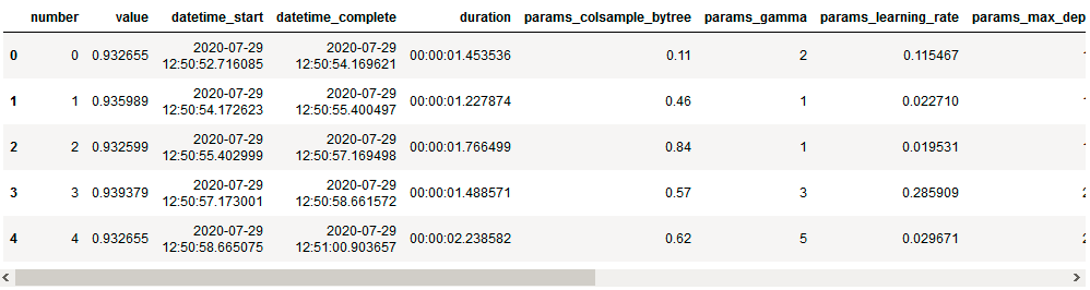
5. Trail History : We can get the entire history of all the trial in the form data frame by just calling study.trails_dataframe().

6. Visualizations :

Photo by Isaac Smith on Unsplash Visualizing the hyperparameter search space can be very useful. From the visualization, we can gain some useful information on the interaction between parameters and we can see where to search next. The optuna.visualization module includes a set of useful visualizations. i) plot_optimization_history(study): plots optimization history of all trials as well as the best score at each point. 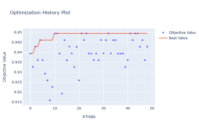Optimization History Plot ii) plot_slice(study): plots the parameter relationship as slice also we can see which part of search space were explored more. 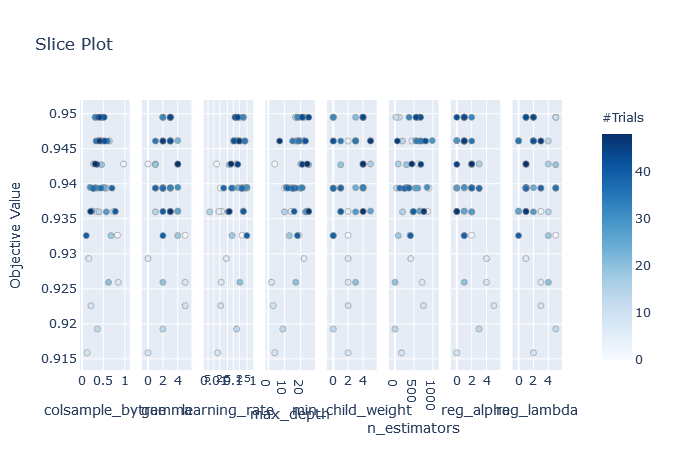Slice Plot iii) plot_parallel_coordinate(study) : plots the interactive visualization of the high-dimensional parameter relationship in study and scores. 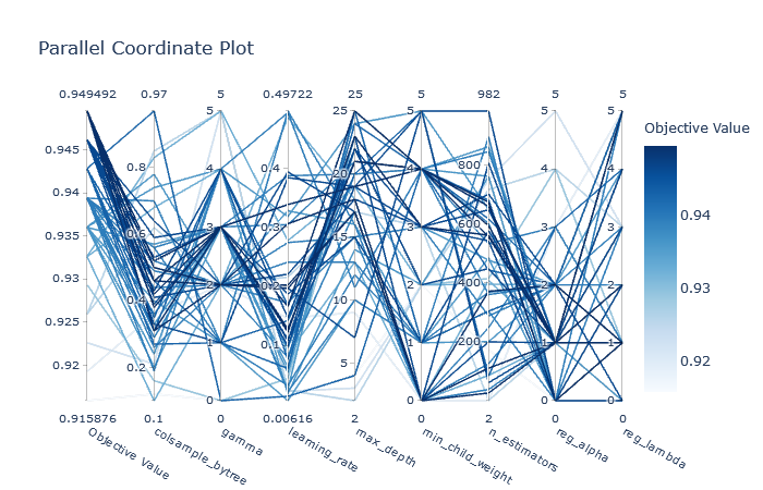Parallel Coordinate Plot iv) plot_contor(study): plots parameter interactive chart from we can choose which hyperparameter space has to explore. 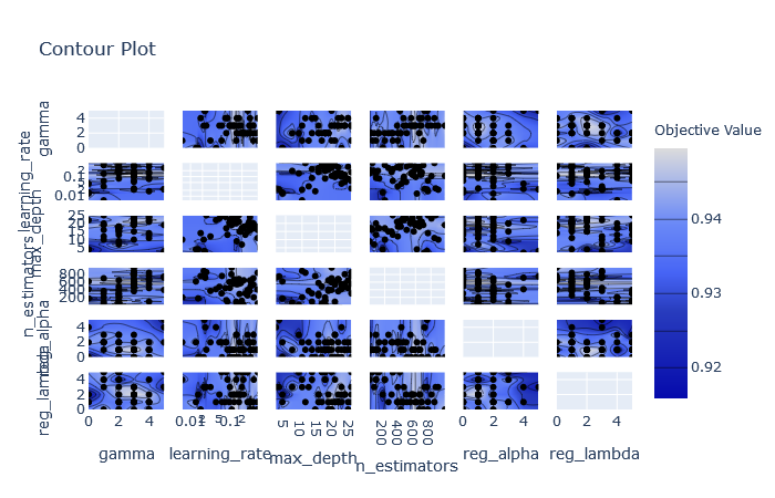Contour Plot Overall, Visualizations are Amazing in Optuna !! Want to see AI/ML models in action?